An International Journal
Agricultural and Biological Research
ISSN - 0970-1907
RNI # 24/103/2012-R1
RNI # 24/103/2012-R1
Research Article - (2025) Volume 41, Issue 4
The issue of plant pests is a critical area of investigation at present. While numerous chemical solutions are available, their toxic effects make the use of natural enemies a preferable alternative. This article introduces a fractional calculus approach to model the dynamics between mature and immature natural enemies of plant pests. The study discusses the existence and uniqueness of the solution, the non-negativity of the solution and both global and local stability of the equilibrium point. Given that memory is intrinsic to biological systems, the proposed technique is advantageous due to the memory effect of fractional derivatives, leading to more accurate solutions. Simulations with different fractional parameters generate optimal solutions.
Fractional differential; Plant pest natural enemy; Numerical simulations
In the present era, the plant-pest problem is a significant global issue. Discussions about plant pests date back to the early 18th century, with George and Watt addressing the pests and delights of tea plants in 1898 and Hilderic Friend studying worms as plant pests in 1911 [1,2]. Over time, many authors have proposed solutions to plant-pest problems, including chemical solutions, biological enemies and pest infections.
Numerous chemical solutions have been explored. For instance, Choo Ho, et al. discussed the effects of some chemical pesticides in 1998 and Hajji et al. examined nanobased pesticides in 2021 [3,4]. However, chemical solutions can sometimes be harmful to both plants and humans. BN Aloo et al. highlighted the adverse effects of agrochemicals on beneficial plant rhizobacteria in agricultural systems in 2021 [5].
Biological enemies are a preferable solution to plant-pest problems. The study of biological control began in 1888 when the Vedalia bug was introduced in California from Australia [6]. Paul DeBach and David Rosen’s 1991 book on biological control explains how natural enemies can biologically control pest populations [7]. In 1995, Thomas et al. published research on the biological control of grasshoppers by fungi [8].
Mathematical modeling of plant-pest interactions has gained traction in recent years. Haith et al. studied models for pest management in the analysis of potato integration in 1987 [9]. Maiti et al. developed a mathematical model on the usefulness of biocontrol for pests in tea in 2008 [10]. Kumar et al. investigated a mathematical model on plant pests and natural enemies with twin gestation delays as a biological control technique in 2018. Many researchers have attempted to construct robust models by addressing various real-world challenges to mitigate flaws in predator-prey relationship models.
Currently, many plant-pest models are developed using ordinary differential equations with various parameters, including delay, harvesting, etc. The fractional differentiation approach for plant-pest models is a new research area. Fractional differentiation introduces a memory effect, which is a valuable criterion for solving plant-pest problems. Bhattacharya et al. studied a fractional differential approach with memory for the paradox of enrichment in 2013. Samanta et al. developed a fractional-order preypredator model incorporating prey in 2018 and Moustafa et al. wrote a paper on a fractional-order prey-predator model in 2019.
Several definitions of fractional differential equations exist, including Grunwald-Letnikov, Riemann-Liouville and Caputo. Among these, Caputo’s fractional derivative is the most popular and well-developed, with initial conditions similar to those for integerorder derivatives.
Recently, researchers have increasingly focused on fractional differentiation due to its memory terms and properties. Caputo fractional derivatives have gained interest for their applications in modeling pandemics like COVID-19, electrical engineering, biochemistry (e.g., modeling proteins and polymers), acoustics, material modeling, rheology and mechanical systems. The fundamental properties and applications of fractional derivatives can be found in the works. Given that memory is inherent in biological systems, fractional derivatives are particularly relevant. This is why I am studying a fractional-order plant-pest model involving immature and mature biological enemies. For fractional differential based model one can cite the following papers.
In this research paper, we discussed a fractional-order differential model for plant pest mature and immature biological enemies.
Using a fractional derivative, we examined the food chain dynamics of plant pests with their immature and mature biological enemies in this work. In this case, we presented the following mathematical approach:
Plant pest premature-mature biological enemy
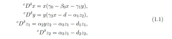
With initial conditions: x (0)>0, y (0)>0, z1(0)>0 and z2(0)>0.
The following is a summary of our work: We reviewed some basic fractional derivative definitions in the preliminaries section. The existence and uniqueness results for the system (1.1) are derived in the main results section. For the system (1.1), the equilibrium points and their stability analysis are also performed. Numerical analysis is performed at the end of this work using matlab code fde12 for fractional differential equations.
Preliminaries
We will review certain terminology and basic fractional calculus results in this section, this will be used for the duration of the research.
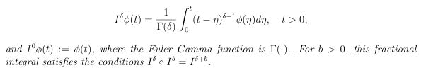
Definition: The fractional integral of a function Φ with order δ>0 lower bound zero is defined as follows.
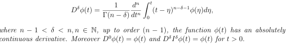
Definition: The Riemann-Liouville fractional derivative of a function Φ with the lower limit zero of order δ>0 is given by
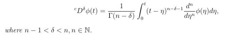
Definition: The caputo fractional derivative of a function Φ ∈ Cn ([0,∞)) with the lower limit zero of order δ>0 is given by
Consider the system
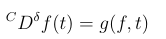
with the initial condition: f(t0)=ft0, where δ ∈ (0,1], g: Γ × [t0, ∞) → Rn,Γ ⊂ Rn, if g(f,t) satisfies the local Lipschitz condition with respect to f, then there exist a unique solution of (2.1) on Γ × [t0, ∞).
Existence and uniqueness
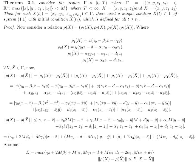
As a result, ρ(X) satisfies the Lipschitz condition with regard to X and hence there exists a unique solution X(t) for system.
Non-negativity and uniform boundedness
The solutions of the system which (1.1) starts in R4 + and non-negative and uniform bounded. Proof. Applied the results used in. Suppose
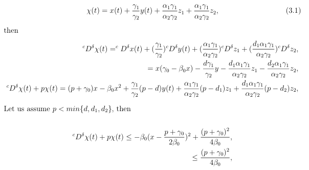
Now applying the comparison theorem for fractional order, one reach
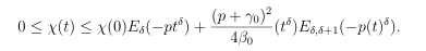
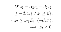
Where Eδ and Eδ, δ+1 are mittag leffler function. Now by taking t → ∞ one get
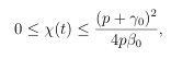
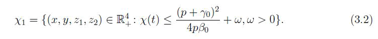
Hence, the solutions of system of fractional differential equation begins i n R4+ are uniformly bounded with in the region χ1 defined as
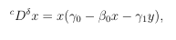
Now we will prove that the solution of fraction order system is non-negative. Consider the first equation of system of equation.
From equation 3.1 and 3.2 and considering ω → 0 one get
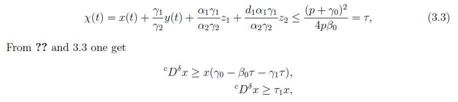
where τ1=(γ0−β0τ−γ1τ), from comparison theorem of one get
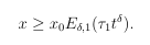
Hence x ≥ 0. Now on taking equation 2 of system 1.1 and 3.1 one get
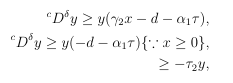
where τ2=d+α1τ, Hence
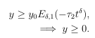
Now considering the equation 3 of system of equation 1.1 one get
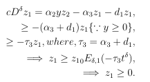
Again from equation 4 of system of equation 1.1 one get
Hence the system of equation 1.1 have non-negative solutions.
Basic reproduction number
For finding equilibrium points and their stability we will introduce basic reproduction with the help of pest free equilibrium point of system of equation.
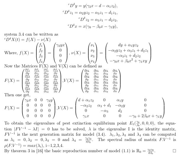
Theorem: The basic reproduction number R0 for the system of equation (1.1) is given by R0=γ2γ0/dβ0.
Proof: Rewriting the given system of equation (1.1)
Steady state points
Local stability analysis
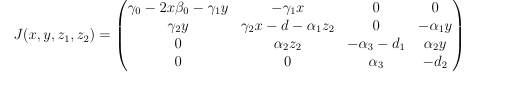
The fundamental matrix for the given system of equation (1.1)
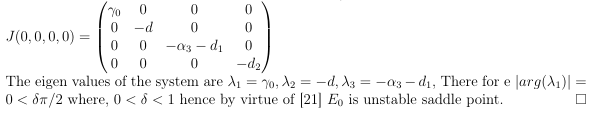
The equilibrium point E0 (0, 0, 0, 0) of system (1.1) is unstable saddle point.
Proof. The Jacobian matrix for equilibrium point E0 is
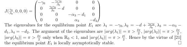
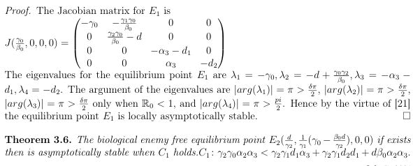
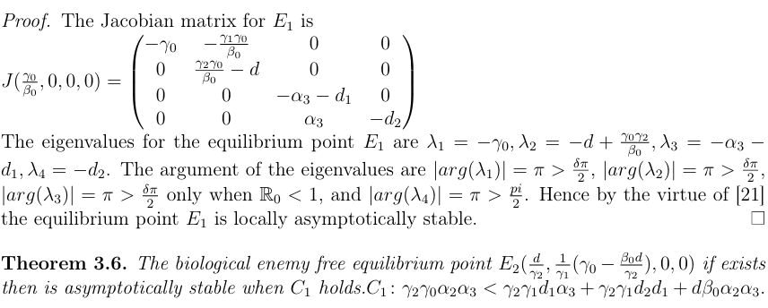
The equilibrium point E1 (γ0/β0, 0, 0, 0) is locally a symptotically stable, when the basic reproduction number R0<1
Numerical analysis
In this section we have developed some graphs of the system (1.1) by using Matlab code FDE12. We will use the values of the parameter as mentioned in the Table 1 and initial value of the population is taken as [x(0), y(0), z1 (0), z2(0)]=[1, 1, 1, 1].
| Para.↓ | Coll | Col2 | Col3 | Col4 |
| γo | 0.9 | 0.9 | 0.9 | 0.3 |
| γ1 | 0.1 | 0.1 | 0.1 | 0.1 |
| γ2 | 0.02 | 0.2 | 0.2 | 0.2 |
| α1 | 0.3 | 0.3 | 0.3 | 0.3 |
| α2 | 0.1 | 0.1 | 0.25 | 0.1 |
| α3 | 0.25 | 0.25 | 0.25 | 0.25 |
| β0 | 0.1 | 0.1 | 0.1 | 0.1 |
| d | 0.2 | 0.2 | 0.2 | 0.2 |
| d1 | 0.1 | 0.1 | 0.2 | 0.1 |
| d2 | 0.2 | 0.2 | 0.1 | 0.2 |
TABLE 1 A table for the various values of parameters used in system (1.1)
Pest extinction point
Taking the values of parameters as defined in column-1 of Table 1, one can observe that the progress rate of pest population (γ2=0.02) is very less than the other cases and the basic reproduction number R0=0.9<1 then we get the pest extinction equilibrium point which is shown in following graphs (Figures 1 and 2).

Figure 1) Time series graph of pest extinction equilibrium point E0 (9, 0, 0, 0) for δ=1, this graph shows that when there is no pest and biological enemy then plant population is higher than the other cases as discussed in this paper

Figure 2) Set of point of state space for the system 1.1, for the different values of fractional parameter δ=1, 0.97, 0.94, 0.91 as defined in Table 1
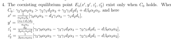
Coexisting point
One can observe from column-2 of Table 1 that when we take γ2=0.2 then we get the R0=9>1 which shows the existence of coexisting equilibrium point (Figures 3-5).

Figure 3) Time series graph of coexisting equilibrium point E3 (6.2, 2.8, 2.7733, 3.4667) for δ=1, and one can observe from the graph that the plant population in presence of pest and biological enemy is higher than the situation when there are no biological enemies and is lesser to the situation when there is no pest and biological enemy both

Figure 4) Set of point of state space for the system 1.1, for coexisting equilibrium for the different values of fractional parameter δ=1, 0.97, 0.94, 0.91 as defined in column-2 of Table 1

Figure 5) Portrait diagram of the model for δ=0.97 with reference to the column-2 of Table 1
Unstable coexisting point
One can observe from column-3 of Table 1 that if one takes the mortality rate (d1=0.2) of immature biological enemy higher than the mortality rate (d2=0.1) of mature biological enemy and the progress rate of immature biological enemy (α2=0.25) then the basic reproduction number is R0=9>1 the coexisting equilibrium point becomes unstable (Figures 6-8).

Figure 6) Time series graph of unstable coexisting equilibrium point E3 (8.9724, 0.0228, 0.2802, 5.0282) for δ=1 and other parameters as defined in column-3 of Table 1

Figure 7) Set of point of state space for the system 1.1, for unstable coexisting equilibrium for the different values of fractional parameter δ=1, 0.97, 0.94, 0.91 and other parameters as defined in column-3 of Table 1

Figure 8) Portrait diagram of the model (1.1) for δ=0.97 with reference to the column-3 of Table 1
Biological enemy free point
One can observe from the column-4 of Table 1 that when the growth rate plants (γ0=0.3) is less than the other cases then R0=3>1 this shows that there is an existence of pest population but one gets the biological enemy free equilibrium state as shown in the following graphs (Figure 9).

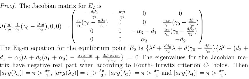
Figure 9) Time series graph of biological enemy free equilibrium point E2 (1, 2, 0, 0) for δ=1
One can see from the graph that the plant population in presence of pest and without biological enemy is lesser than all the cases we discussed in this paper. Hence if there is exist pest in plant than there should by biological enemy for the protection and growth of plants (Figure 10).

Figure 10) Set of point of state space for the system 1.1, for biological enemy free equilibrium for the different values of fractional parameter δ=1, 0.97, 0.94, 0.91 as defined in column-4 of Table 1
In this paper, we presented a result on the existence and uniqueness, of the solution as well as (3.2) on the non-negativity and uniform boundedness for a class of systems under the control of (1.1). The stability of the equilibrium points has been discussed. According to the discussion in (3.4), the equilibrium point E0 is unstable saddle point, the equilibrium point E1 is locally and globally asymptotically stable when the condition R0<1 holds as discussed in 3.5 and 3.8, the equilibrium point E2 is asymptotically stable only when the condition C1 holds as discussed in 3.6 and the equilibrium point E3 is also locally and globally asymptotically stable If C2 holds as discussed in 3.7. In the end, equilibrium points are numerically analysed as explained in (4). From the numerical simulation, it can be seen that fractional order changes the convergence speed of the solution of fractional differential system and it is also seen when fractional order δ increases (0<δ<1) the convergence speed of solution is also increased which shows the memory term of fractional order.
The labelled dataset used to support the findings of this study is available from the corresponding author on request.
[Crossref] [Google Scholar] [PubMed]
Received: 07-Jul-2024, Manuscript No. AGBIR-24-140957; , Pre QC No. AGBIR-24-140957 (PQ); Editor assigned: 09-Jul-2024, Pre QC No. AGBIR-24-140957 (PQ); Reviewed: 23-Jul-2024, QC No. AGBIR-24-140957; Revised: 09-Aug-2025, Manuscript No. AGBIR-24-140957 (R); Published: 16-Aug-2025, DOI: 10.37532/0970-1907.25.41(4):1-7